2-3
Trees
(Up to Basic
Computer Science : Data Trees)
The 2-3 tree is also a search tree like the binary
search tree, but this tree tries to solve the problem of the unbalanced tree.
Imagine that you have a binary tree to store your data. The worst
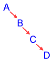
possible case for the binary tree is that all of the data is entered in order. Then the tree would look like this:

This tree has basically turned into a linked
list. This is definitely a problem, for with a tree unbalanced
like this, all of the advantages of the binary search tree disappear:
searching the tree is slow and cumbersome, and there is much wasted memory because of the empty left child pointers.
The 2-3 tree tries to solve this by using a different structure
and slightly different adding and removing procedure to help keep
the tree more or less balanced. The biggest drawback with the 2-3
tree is that it requires more storage space than the normal binary
search tree.
The 2-3 tree is called such because the maximum possible number
of children each node can have is either 2 or 3. This makes the
tree a bit more complex, so I will try to explain as much as possible.
One big difference with the 2-3 tree is that each node can have
up to two data fields. You can see the three children extending from between the two data fields.

Thus, the tree is set up in the following manner:
- The node must always have a first field (data 1 in the
diagram ), but not necessarily a second field (data 2).
If both fields are present in a node, the first (or left) field
of the node is always less than the second (or right) field of
the node.
- Each node can have up to three child nodes, but if there is
only one data field in the node, the node cannot have more than
two children.
- The child nodes are set so that data in the first sub-tree is
less than the first data field, the data of the second sub-tree
is greater than the first data field and less than the second
data field, and the data of the third sub-tree is greater than
the second data field. If there is only one data field in the
node, use the first and second children only.
- All leaf nodes appear on the last level.
Now, take a look at the implementation of a 2-3 tree:
class twoThreeTree {
public:
twoThreeTree(void);
~twoThreeTree(void);
void add(int item);
void search(int item);
private:
twoThreeNode *root;
};
class twoThreeNode {
public:
int firstData, secondData;
twoThreeNode *first, *second, *third;
twoThreeNode *parent;
};
You can see that this tree, unlike the binary
search tree or the heap tree, has no remove() function. It is possible
to program a remove function, but it generally isn't worth the time
nor the effort.
This tree will be a bit harder to implement than the binary search
tree just because of the complexity of the node. Still, the add()
function algorithm isn't that difficult, and a step-by-step
progression throug the algorithm helps enormously.
First, to add an item, find the place in the tree for it. This
is very much the same as in the binary search tree: just compare
and move down the correct link until leaf node is reached.
Once at the leaf node, there are three basic cases for the add()
function:
- The leaf node has only one data item: this case is very
simple. Just insert the new item after this item or shift the
old item forward and insert the new item before the old one, depending
on the situation.
- The leaf node is full and the parent node has only one data
item: this case is also quite simple. Compare the three values:
the two leaf node items and the new item. Choose the middle one
and insert it in the parent node where appropriate
If the leaf node is the left child, shift the old data in the
parent node to the right and insert the middle value in the parent
node before the old data. Make sure to shift the pointers to
the children in the parent node! If the leaf is the right
child, just insert the middle value to the right of the old value
in the parent node. The two left-over values from the comparison
become two leaf nodes, one as the second child, and one as the
first or third child depending on the situation.
- Both the leaf node and the parent node are full: this
situation is the most complex of all. In the same manner as Case
2, promote the middle value of the leaf node. Then, continue doing
the same thing with the parent node, and so on until the situation
is resolved or the root node is reached. In this case, the middle
value is promoted once again, except a new root node is created
from the middle value and the two other values become the left
and right subtrees of the new root. At the leaf node at which
we began, the new level allows us to split the three initial values
into a three node sub-tree of the parent node...etc.
Doing a few small 2-3 trees by hand helps to understand
this algorithm. Remember to check and hold to the rules governing
the 2-3 tree! It can get ugly if they are ignored, especially
with the last one.
Using some recursive helper functions as well as that miraculous parent variable will help ease the pain
of programming this tree.

